How To Find The Characteristic Polynomial Of A 3x3 Matrix
Juapaving
Mar 23, 2025 · 5 min read
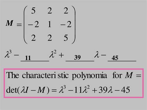
Table of Contents
How to Find the Characteristic Polynomial of a 3x3 Matrix
Finding the characteristic polynomial of a matrix is a fundamental concept in linear algebra with applications spanning diverse fields like physics, engineering, and computer science. This comprehensive guide will walk you through the process of determining the characteristic polynomial for a 3x3 matrix, explaining the underlying theory and providing practical examples. We'll cover multiple methods, ensuring you grasp the concept thoroughly.
Understanding the Fundamentals
Before diving into the calculations, let's establish a solid foundation. The characteristic polynomial is a polynomial whose roots are the eigenvalues of the matrix. Eigenvalues are scalar values that, when multiplied by a vector (eigenvector), result in the same vector being scaled by that scalar. In simpler terms, they represent how a linear transformation stretches or shrinks vectors.
The characteristic polynomial is defined as:
det(A - λI) = 0
Where:
- A is the 3x3 matrix.
- λ (lambda) represents the eigenvalues.
- I is the 3x3 identity matrix (a matrix with 1s on the main diagonal and 0s elsewhere).
- det() denotes the determinant of the matrix.
This equation states that the determinant of the matrix (A - λI) must be zero for the eigenvalues to be found. The determinant of (A - λI) itself is the characteristic polynomial.
Method 1: Direct Calculation of the Determinant
This method involves directly calculating the determinant of (A - λI). While seemingly straightforward, it can become computationally intensive for larger matrices. For a 3x3 matrix, it's manageable.
Let's consider a sample 3x3 matrix A:
A = | 2  1  0 |
    | 1  2  1 |
    | 0  1  2 |
Step 1: Subtract λI from A
First, subtract λI from A:
A - λI = | 2-λ  1   0 |
         |  1  2-λ  1 |
         |  0   1  2-λ |
Step 2: Calculate the Determinant
Now, compute the determinant of (A - λI). Remember the formula for the determinant of a 3x3 matrix:
det(A - λI) = (2-λ)[(2-λ)(2-λ) - 1] - 1[(2-λ) - 0] + 0
Step 3: Simplify the Polynomial
Expand and simplify the expression to obtain the characteristic polynomial:
det(A - λI) = (2-λ)[(4 - 4λ + λ²) - 1] - (2-λ)
             = (2-λ)(3 - 4λ + λ²) - (2-λ)
             = (2-λ)(2 - 4λ + λ²)
             = -λ³ + 6λ² - 11λ + 6
Therefore, the characteristic polynomial for matrix A is -λ³ + 6λ² - 11λ + 6 = 0. The roots of this polynomial (the eigenvalues) can then be found using various methods like the rational root theorem or numerical methods.
Method 2: Using Eigenvalue Properties
This method leverages properties of eigenvalues to simplify the calculation. While not directly calculating the determinant, it offers a more insightful approach.
Step 1: Trace and Determinant
The trace of a matrix (tr(A)) is the sum of its diagonal elements. The determinant of a matrix, as we already know, is a scalar value. For a 3x3 matrix, the characteristic polynomial can be expressed as:
λ³ - tr(A)λ² + (sum of principal 2x2 minors)λ - det(A) = 0
Let's use the same matrix A from the previous example:
- tr(A) = 2 + 2 + 2 = 6
- det(A) = 2(4 - 1) - 1(2 - 0) + 0 = 6
The sum of principal 2x2 minors is calculated as follows:
- Minor 1: (22 - 11) = 3
- Minor 2: (22 - 00) = 4
- Minor 3: (22 - 11) = 3
- Sum of minors: 3 + 4 + 3 = 10
Step 2: Construct the Polynomial
Substitute these values into the polynomial equation:
λ³ - 6λ² + 11λ - 6 = 0 (Note the slight difference from Method 1 due to coefficient order)
This is the characteristic polynomial, the same as before, although the order of coefficients may vary slightly depending on the method of expansion.
Method 3: Leveraging Software Tools
For larger matrices or complex calculations, software packages like MATLAB, Python's NumPy, or Wolfram Mathematica significantly simplify the process. These tools possess built-in functions for calculating the characteristic polynomial.
For instance, in Python with NumPy:
import numpy as np

A = np.array([[2, 1, 0], [1, 2, 1], [0, 1, 2]])
p = np.poly(A) # p will contain the coefficients of the characteristic polynomial.
print(p)
This will output the coefficients of the characteristic polynomial. Remember to interpret the output coefficients correctly to obtain the polynomial in the standard form.
Applications of the Characteristic Polynomial
The characteristic polynomial is not just a theoretical concept; it finds practical application in numerous areas:
-
Eigenvalue Problems: The most direct application is finding the eigenvalues of a matrix, which are crucial in understanding the behavior of linear systems. Eigenvalues represent scaling factors in linear transformations.
-
Stability Analysis: In control systems and dynamical systems, the eigenvalues determine the stability of the system. If the real parts of all eigenvalues are negative, the system is stable.
-
Diagonalization: The characteristic polynomial helps determine whether a matrix is diagonalizable. A matrix is diagonalizable if its algebraic multiplicity (the multiplicity of the eigenvalue as a root of the characteristic polynomial) equals its geometric multiplicity (the dimension of the eigenspace associated with the eigenvalue).
-
Matrix Decomposition: The characteristic polynomial contributes to various matrix decompositions like the Jordan canonical form, which is essential in solving systems of differential equations.
-
Quantum Mechanics: In quantum mechanics, the characteristic polynomial of the Hamiltonian operator helps determine the energy levels of a quantum system.
-
Graph Theory: The characteristic polynomial of an adjacency matrix of a graph provides information about the graph's structure and properties.
Advanced Considerations
-
Complex Eigenvalues: Matrices can have complex eigenvalues. The characteristic polynomial remains valid even in these cases.
-
Repeated Eigenvalues: When eigenvalues are repeated (have algebraic multiplicity greater than 1), it's crucial to determine their geometric multiplicity to fully characterize the matrix.
-
Numerical Methods: For larger matrices, numerical methods are essential for finding the roots of the characteristic polynomial, as analytical solutions become intractable.
Conclusion
Finding the characteristic polynomial of a 3x3 matrix, though involving some algebraic manipulation, provides the key to unlocking vital information about the matrix itself and its corresponding linear transformation. Mastering this process opens the door to understanding eigenvalue problems, analyzing system stability, and delving into more advanced concepts within linear algebra and its diverse applications in numerous fields. Remember to practice consistently to strengthen your understanding and skills. Remember to always check your work meticulously as even small mistakes in calculation can significantly alter the result.
Latest Posts
Latest Posts
-
What Is The Molecular Mass Of Calcium Nitrate
Mar 24, 2025
-
Least Common Multiple Of 12 And 13
Mar 24, 2025
-
Matter Is Anything That Has Mass And
Mar 24, 2025
-
Two Pairs Of Opposite Parallel Sides
Mar 24, 2025
-
Least Common Multiple Of 10 15 And 25
Mar 24, 2025
Related Post
Thank you for visiting our website which covers about How To Find The Characteristic Polynomial Of A 3x3 Matrix . We hope the information provided has been useful to you. Feel free to contact us if you have any questions or need further assistance. See you next time and don't miss to bookmark.
