How To Calculate Eigenvectors From Eigenvalues
Juapaving
Mar 24, 2025 · 5 min read
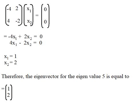
Table of Contents
How to Calculate Eigenvectors from Eigenvalues: A Comprehensive Guide
Eigenvectors and eigenvalues are fundamental concepts in linear algebra with widespread applications in various fields, including physics, engineering, computer science, and data science. Understanding how to calculate eigenvectors from eigenvalues is crucial for leveraging their power in these domains. This comprehensive guide will walk you through the process, explaining the underlying theory and providing step-by-step examples.
Understanding Eigenvalues and Eigenvectors
Before diving into the calculations, let's solidify our understanding of the core concepts:
Eigenvalues: These are scalar values that represent how much a linear transformation stretches or shrinks a vector. They are often denoted by λ (lambda).
Eigenvectors: These are non-zero vectors that, when transformed by a linear transformation (represented by a matrix), only change in scale (magnitude), not direction. They remain aligned with their original direction.
The relationship between eigenvalues and eigenvectors is defined by the following equation:
Av = λv
Where:
- A is the square matrix representing the linear transformation.
- v is the eigenvector.
- λ is the eigenvalue.
This equation states that when the matrix A acts on the eigenvector v, the result is a scaled version of the same eigenvector v, scaled by the eigenvalue λ.
The Process of Calculating Eigenvectors
Calculating eigenvectors involves a multi-step process:
-
Finding the Eigenvalues: First, we need to determine the eigenvalues of the matrix A. This involves solving the characteristic equation:
det(A - λI) = 0
Where:
- det() denotes the determinant of a matrix.
- I is the identity matrix (a square matrix with 1s on the main diagonal and 0s elsewhere).
Solving this equation yields the eigenvalues λ₁, λ₂, etc.
-
Solving for Each Eigenvector: For each eigenvalue λᵢ, we need to solve the following equation:
(A - λᵢI)vᵢ = 0
This is a system of homogeneous linear equations. The solution to this system will give us the eigenvector vᵢ corresponding to the eigenvalue λᵢ. Note that this system will always have infinitely many solutions, as any scalar multiple of an eigenvector is also an eigenvector. Therefore, we usually normalize the eigenvector to have a length of 1.
Step-by-Step Examples
Let's illustrate the process with a few examples of increasing complexity:
Example 1: A 2x2 Matrix
Consider the matrix:
A =  [[2, 1],
     [1, 2]]
1. Finding the Eigenvalues:
The characteristic equation is:
det(A - λI) = det([[2-λ, 1], [1, 2-λ]]) = (2-λ)² - 1 = 0
Solving this quadratic equation gives us two eigenvalues:
λ₁ = 3 λ₂ = 1
2. Solving for the Eigenvectors:
-
For λ₁ = 3:
(A - 3I)v₁ = 0 => [[-1, 1], [1, -1]]v₁ = 0
This simplifies to -x + y = 0, which means x = y. Let's choose x = 1, then y = 1. Therefore, v₁ = [[1], [1]]. We can normalize this eigenvector:
v₁ = [[1/√2], [1/√2]]
-
For λ₂ = 1:
(A - I)v₂ = 0 => [[1, 1], [1, 1]]v₂ = 0
This simplifies to x + y = 0, which means x = -y. Let's choose x = 1, then y = -1. Therefore, v₂ = [[1], [-1]]. Normalizing this eigenvector:
v₂ = [[1/√2], [-1/√2]]
Example 2: A 3x3 Matrix
Let's consider a slightly more complex 3x3 matrix:
A = [[2, 0, 0],
     [0, 3, 4],
     [0, 4, -3]]
1. Finding the Eigenvalues:
The characteristic equation is:
det(A - λI) = det([[2-λ, 0, 0], [0, 3-λ, 4], [0, 4, -3-λ]]) = (2-λ)((3-λ)(-3-λ) - 16) = 0
This gives us three eigenvalues:
λ₁ = 2 λ₂ = 5 λ₃ = -5
2. Solving for the Eigenvectors:
The process is similar to the previous example, but with three equations for each eigenvalue. Solving each system of equations will yield the corresponding eigenvectors. This often involves using techniques like Gaussian elimination or row reduction. For instance, for λ₁=2:
(A - 2I)v₁ = 0 => [[0, 0, 0], [0, 1, 4], [0, 4, -5]]v₁ = 0
This will lead to a solution for v₁. The same procedure should be repeated for λ₂ and λ₃.
Example 3: Cases with Repeated Eigenvalues (Degeneracy)
When a matrix has repeated eigenvalues, finding the eigenvectors can be more challenging. This scenario might lead to a system of equations with fewer independent equations than unknowns, resulting in multiple linearly independent eigenvectors.
Let's imagine a matrix with a repeated eigenvalue λ = 2 with algebraic multiplicity 2 (meaning the eigenvalue appears twice in the characteristic equation). The process of finding the eigenvectors remains the same, but you might end up with a one-dimensional eigenspace (only one linearly independent eigenvector) or a two-dimensional eigenspace (two linearly independent eigenvectors) for this repeated eigenvalue, depending on the matrix.
Advanced Techniques and Considerations
For larger matrices, manual calculation becomes impractical. Numerical methods and computational tools are essential. Software packages like MATLAB, Python's NumPy and SciPy libraries, and others provide functions for efficiently calculating eigenvalues and eigenvectors.
Furthermore, understanding concepts like algebraic multiplicity (how many times an eigenvalue is a root of the characteristic polynomial) and geometric multiplicity (the dimension of the eigenspace associated with an eigenvalue) is crucial when dealing with repeated eigenvalues and degenerate cases. These concepts inform the number of linearly independent eigenvectors you should expect for each eigenvalue.
Applications of Eigenvalues and Eigenvectors
The applications of eigenvalues and eigenvectors are vast and impactful:
-
Principal Component Analysis (PCA): In data science and machine learning, PCA uses eigenvectors of the covariance matrix to reduce the dimensionality of data while preserving maximum variance.
-
PageRank Algorithm (Google Search): The ranking of web pages in Google's search results utilizes the eigenvector corresponding to the largest eigenvalue of a matrix representing links between web pages.
-
Stability Analysis of Dynamical Systems: In engineering and physics, eigenvalues determine the stability of systems. For instance, the eigenvalues of a system's state matrix indicate whether the system will converge to a steady state or diverge.
-
Image Compression and Signal Processing: Eigenvectors play a significant role in techniques like singular value decomposition (SVD), which is applied to compress images and process signals efficiently.
Conclusion
Calculating eigenvectors from eigenvalues is a cornerstone of linear algebra and has profound implications across diverse scientific and technological fields. While the fundamental process involves solving a system of linear equations derived from the eigenvalue equation, the complexity can vary depending on the size of the matrix and the presence of repeated eigenvalues. Mastering this skill empowers you to tackle intricate problems and unlock the potential of this powerful mathematical tool. Remember to leverage computational tools for larger matrices and to delve deeper into advanced concepts like algebraic and geometric multiplicity to fully grasp the nuances of eigenvectors and eigenvalues.
Latest Posts
Latest Posts
-
Three Equivalent Fractions For 3 8
Mar 26, 2025
-
How To Determine Grams From Moles
Mar 26, 2025
-
What Is The Square Root Of 23
Mar 26, 2025
-
How Many Chromosomes Does A Human Gamete Have
Mar 26, 2025
-
Whats The Smallest Organ In The Human Body
Mar 26, 2025
Related Post
Thank you for visiting our website which covers about How To Calculate Eigenvectors From Eigenvalues . We hope the information provided has been useful to you. Feel free to contact us if you have any questions or need further assistance. See you next time and don't miss to bookmark.
