Find The Area Under The Curve Calculator
Juapaving
Mar 30, 2025 · 7 min read
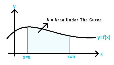
Table of Contents
Find the Area Under the Curve Calculator: A Comprehensive Guide
Finding the area under a curve is a fundamental concept in calculus with wide-ranging applications in various fields, from physics and engineering to economics and statistics. Manually calculating these areas can be complex and time-consuming, especially for intricate functions. This is where an area under the curve calculator becomes invaluable. This comprehensive guide explores the concept, its applications, the different methods used by calculators, and how to effectively utilize these tools.
Understanding the Area Under the Curve
The area under a curve, more formally known as definite integral, represents the accumulated value of a function over a specific interval. Visually, it's the area bounded by the curve, the x-axis, and two vertical lines representing the limits of integration.
Why is this important? The area under the curve provides crucial information depending on the context of the function:
- Physics: Calculating the distance traveled by an object given its velocity function over time.
- Engineering: Determining the total work done by a force over a certain displacement.
- Economics: Calculating the total revenue generated over a period given a demand function.
- Statistics: Finding the probability of an event occurring within a specific range given a probability density function.
Methods for Calculating the Area Under the Curve
Several methods exist for calculating the area under a curve, ranging from simple geometric approaches to sophisticated numerical techniques. Area under the curve calculators typically employ these methods:
1. Geometric Methods:
This approach is applicable to simple functions where the area can be easily determined using basic geometric shapes like rectangles, triangles, and trapezoids. For instance:
- Rectangles: If the function is a constant, the area is simply the product of the base (interval width) and the height (function value).
- Triangles: For linear functions, the area can be calculated using the formula: 0.5 * base * height.
- Trapezoids: For functions that are approximately linear over small intervals, the area can be approximated using trapezoids.
Limitations: Geometric methods are limited to simple functions. They become impractical and inaccurate for complex curves.
2. Numerical Integration Techniques:
Numerical integration techniques are essential for calculating the area under complex curves where analytical solutions are unavailable or difficult to obtain. Calculators often use these methods:
-
Riemann Sums: This method approximates the area by dividing the interval into smaller subintervals and summing the areas of rectangles or other shapes formed by the function values at selected points within each subinterval. Different types of Riemann sums exist, including left Riemann sum, right Riemann sum, and midpoint Riemann sum, each offering varying degrees of accuracy.
-
Trapezoidal Rule: This method improves upon the Riemann sum by approximating the area under the curve using trapezoids instead of rectangles, resulting in a more accurate estimation. It sums the areas of trapezoids formed by connecting adjacent points on the curve.
-
Simpson's Rule: This method offers even greater accuracy by approximating the curve using parabolic segments instead of straight lines. It provides a weighted average of the function values at equally spaced points.
-
Gaussian Quadrature: A more sophisticated technique that uses strategically chosen points and weights to achieve high accuracy with a smaller number of function evaluations. It's especially efficient for smooth functions.
Accuracy & Number of Subintervals: The accuracy of numerical integration techniques depends on the number of subintervals used. More subintervals generally lead to higher accuracy but also increased computation time. Area under the curve calculators usually allow users to adjust the number of subintervals to control the accuracy of the approximation.
Using an Area Under the Curve Calculator
While the underlying mathematical principles are important, the beauty of an area under the curve calculator lies in its simplicity and ease of use. Most calculators follow a similar workflow:
-
Input the Function: Enter the mathematical expression representing the function whose area you want to calculate. Pay close attention to the syntax, ensuring it's correctly formatted according to the calculator's requirements. Common notations and functions should be supported, such as trigonometric functions (sin, cos, tan), exponential functions (e^x), logarithmic functions (ln, log), and others.
-
Specify the Limits of Integration: Define the interval over which you want to calculate the area. These are the lower and upper bounds of the integration. The calculator needs these limits to define the area to be calculated.
-
Select the Method (If Applicable): Some calculators may allow you to select the numerical integration method (e.g., Riemann sum, Trapezoidal rule, Simpson's rule). For most purposes, the default method is sufficient, but understanding the options empowers more refined calculations when needed.
-
Set the Number of Subintervals (If Applicable): For numerical integration methods, you might be able to adjust the number of subintervals. A larger number generally leads to better accuracy, but it might also increase the processing time. Experimentation can help you find a balance between accuracy and speed.
-
Obtain the Result: Once you've provided all the necessary inputs, click the "Calculate" button, and the calculator will compute the area under the curve. The result will be displayed, usually with a specified number of decimal places.
Applications of Area Under the Curve Calculation
The ability to calculate the area under the curve has widespread applications across numerous disciplines:
1. Physics:
- Calculating displacement from velocity: If you have a graph of an object's velocity over time, the area under the curve represents the total distance traveled by the object.
- Determining work done: The area under a force-displacement curve represents the total work done by the force.
- Finding total impulse: The area under a force-time curve represents the total impulse experienced by an object.
2. Engineering:
- Analyzing stress-strain curves: The area under a stress-strain curve represents the energy absorbed by a material before failure. This is crucial in material science and structural engineering.
- Calculating fluid flow: In fluid dynamics, the area under certain curves can represent flow rates or other important quantities.
3. Economics:
- Calculating consumer surplus: In economics, the area under the demand curve and above the market price represents the consumer surplus. This represents the total benefit consumers receive from purchasing a good or service at the market price.
- Calculating producer surplus: The area under the market price and above the supply curve represents the producer surplus, the benefit producers receive from selling goods or services.
- Estimating total revenue: The area under a revenue function over a specific time period represents the total revenue.
4. Statistics and Probability:
- Finding probabilities: The area under a probability density function (PDF) within a given range represents the probability that a random variable falls within that range. This is fundamental in statistical analysis and modeling.
- Calculating expected values: The area under a weighted function represents the expected value of a random variable.
5. Other Applications:
- Medicine: Analyzing drug concentration levels over time, determining the total drug exposure.
- Environmental Science: Modeling pollutant dispersal, calculating total pollutant emissions.
- Computer Science: Estimating the complexity of algorithms.
Choosing the Right Area Under the Curve Calculator
Several online calculators and software packages are available for computing the area under the curve. When choosing a calculator, consider the following:
- Functionality: Does the calculator support the functions and integration methods you need?
- Ease of use: Is the interface intuitive and easy to navigate?
- Accuracy: Does the calculator provide sufficient accuracy for your purposes? Look for calculators that allow you to adjust the number of subintervals or use more sophisticated integration techniques.
- Documentation: Is there clear documentation explaining how to use the calculator and interpret the results?
Conclusion: Empowering Calculations with Area Under the Curve Calculators
Area under the curve calculations are crucial in many fields. While manual calculation can be challenging for complex functions, online calculators provide a powerful and user-friendly tool to simplify this process. By understanding the underlying methods and effectively utilizing these tools, you can efficiently tackle complex problems and gain valuable insights from your data. Remember to choose a calculator that suits your specific needs in terms of functionality, ease of use, and accuracy. With the right tools and understanding, unlocking the secrets hidden beneath curves becomes straightforward and efficient.
Latest Posts
Latest Posts
-
Area Moment Of Inertia Of A Triangle
Apr 01, 2025
-
What Is The Si Unit Of Kinetic Energy
Apr 01, 2025
-
50 Cm Is Equal To How Many Meters
Apr 01, 2025
-
Difference Between Ac And Dc Examples
Apr 01, 2025
-
How Many Electrons Can The F Sublevel Hold
Apr 01, 2025
Related Post
Thank you for visiting our website which covers about Find The Area Under The Curve Calculator . We hope the information provided has been useful to you. Feel free to contact us if you have any questions or need further assistance. See you next time and don't miss to bookmark.
