What Is A Joint Probability Distribution
Juapaving
Mar 12, 2025 · 8 min read
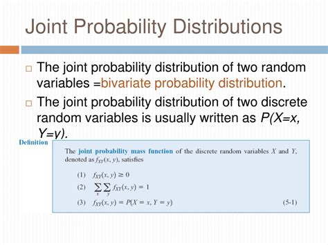
Table of Contents
What is a Joint Probability Distribution? A Comprehensive Guide
Understanding probability distributions is fundamental to many fields, from statistics and machine learning to finance and physics. While individual probability distributions describe the likelihood of a single random variable taking on specific values, joint probability distributions extend this concept to multiple variables, revealing how these variables are related. This comprehensive guide will delve into the intricacies of joint probability distributions, exploring their definitions, types, applications, and practical examples.
Defining Joint Probability Distributions
A joint probability distribution describes the probability of two or more random variables simultaneously taking on specific values. Imagine you're tracking the daily high temperature and the amount of rainfall in a city. A joint probability distribution would tell you the probability of observing, for instance, a high temperature of 25°C and 10mm of rainfall on a given day. This contrasts with individual (marginal) distributions, which would only describe the probability of a specific temperature or rainfall amount independently.
Formally, for discrete random variables X and Y, the joint probability mass function (PMF), denoted as P(X=x, Y=y), gives the probability that X takes the value 'x' and Y takes the value 'y'. For continuous random variables, the joint probability density function (PDF), denoted as f(x,y), describes the probability density at a specific point (x,y). Note that for continuous variables, the probability of the variables taking on exactly specific values is zero; instead, we consider probabilities over intervals.
Key Characteristics of Joint Probability Distributions:
- Non-negativity: The probability of any combination of values must be non-negative (P(X=x, Y=y) ≥ 0 or f(x,y) ≥ 0).
- Normalization: The sum of all probabilities (for discrete variables) or the integral over all possible values (for continuous variables) must equal 1. This reflects the certainty that some outcome will occur.
- Marginal Distributions: We can derive the individual probability distributions of each variable from the joint distribution. This is done by summing (discrete) or integrating (continuous) over the other variable(s). These individual distributions are called marginal distributions.
- Conditional Distributions: Joint distributions allow us to calculate conditional probabilities, such as the probability of a certain temperature given a specific rainfall amount. This involves calculating the probability of one variable given a specific value of the other variable.
Types of Joint Probability Distributions
Several types of joint distributions exist, depending on the nature of the random variables involved and their relationships. Some common types include:
1. Bivariate Normal Distribution:
This is perhaps the most widely used joint distribution, involving two normally distributed random variables. It's characterized by its mean vector (containing the means of both variables) and its covariance matrix (describing the variance of each variable and their covariance—a measure of how they change together). The bivariate normal distribution is crucial in many statistical applications, particularly regression analysis and hypothesis testing. Its bell-shaped surface reflects the probability density across the two variables.
2. Multinomial Distribution:
An extension of the binomial distribution to multiple outcomes, the multinomial distribution describes the probabilities of different outcomes in a series of independent trials, each with more than two possible results. Imagine rolling a six-sided die multiple times; the multinomial distribution models the probabilities of observing various counts of each face.
3. Multivariate Normal Distribution:
This generalizes the bivariate normal distribution to any number of normally distributed variables. It's defined by its mean vector and covariance matrix, which now describe the relationships among all the variables. It’s a cornerstone of multivariate statistical analysis.
4. Joint Discrete Distributions:
This category encompasses numerous distributions where all the variables involved are discrete. Examples include joint distributions involving binomial, Poisson, or geometric random variables. The specific form of the joint PMF will depend on the underlying relationship between the variables.
5. Joint Continuous Distributions:
This encompasses distributions where all variables are continuous. Beyond the bivariate and multivariate normal distributions, we can encounter other types such as joint uniform distributions (where all points within a defined region have equal probability density) or distributions derived from transformations of known distributions.
Calculating Probabilities from Joint Distributions
The way you calculate probabilities differs slightly depending on whether you are working with discrete or continuous variables.
Discrete Variables:
For discrete random variables X and Y, the probability of X=x and Y=y is simply given by the joint PMF: P(X=x, Y=y). For example, if you have a table showing the joint probabilities for different combinations of X and Y, you can directly read off the probability for any specific (x, y) pair.
Continuous Variables:
For continuous variables, the probability of X falling within a certain range and Y within another range is calculated by integrating the joint PDF over those ranges:
∫∫<sub>R</sub> f(x,y) dx dy
where R represents the region of interest in the x-y plane. This integration gives the probability that (X, Y) falls within the specified region R.
Applications of Joint Probability Distributions
Joint probability distributions have a vast array of applications across numerous disciplines:
1. Finance:
Modeling portfolio risk, evaluating investment strategies, pricing derivatives, and understanding correlations between asset prices all heavily rely on joint distributions. For example, the correlation between stock prices can be analyzed using joint distributions to better manage investment portfolios.
2. Machine Learning:
In machine learning, joint distributions are essential for tasks such as Bayesian networks, probabilistic graphical models, and hidden Markov models. These models represent complex relationships between variables using joint probabilities.
3. Meteorology:
Predicting weather patterns often involves joint distributions to model the relationships between temperature, humidity, wind speed, and precipitation. These models help forecasters anticipate extreme weather events.
4. Medical Research:
Joint distributions are used to study the relationship between different health factors, such as blood pressure, cholesterol levels, and the risk of heart disease. This helps researchers understand disease mechanisms and develop effective treatments.
5. Engineering:
Reliability analysis of systems often uses joint distributions to assess the probability of component failures and the overall system's failure rate. This is crucial for designing robust and dependable systems.
Independence and Dependence in Joint Distributions
A crucial aspect of joint distributions is understanding the relationship between the variables involved.
Independent Variables: If two random variables X and Y are independent, their joint distribution is simply the product of their individual (marginal) distributions:
P(X=x, Y=y) = P(X=x) * P(Y=y) (for discrete variables) f(x,y) = f<sub>X</sub>(x) * f<sub>Y</sub>(y) (for continuous variables)
This means the occurrence of one event doesn't affect the probability of the other event. However, many real-world situations involve dependent variables, where the value of one variable influences the probability of the other.
Dependent Variables: When variables are dependent, their joint distribution cannot be factored into the product of their marginal distributions. This dependence is often quantified by measures like covariance or correlation. For instance, the height and weight of individuals are typically positively correlated – taller individuals tend to weigh more. A joint distribution captures this dependence.
Conditional Probability and Joint Distributions
Joint distributions are fundamental to understanding conditional probability. The conditional probability of event A given event B has occurred is given by:
P(A|B) = P(A and B) / P(B)
In the context of random variables X and Y, the conditional probability of X=x given Y=y is:
P(X=x|Y=y) = P(X=x, Y=y) / P(Y=y)
This formula highlights how the joint distribution provides the necessary information to calculate conditional probabilities. The conditional probability describes how the probability of one variable changes when we know the value of another.
Visualizing Joint Probability Distributions
Visualizing joint distributions provides valuable insights into the relationships between variables. Methods include:
-
Scatter plots: For continuous variables, a scatter plot shows the data points (x, y), allowing for visual inspection of relationships (linear, non-linear, or no relationship).
-
Heatmaps: These are particularly useful for discrete or discretized continuous variables. They represent the joint probabilities as colors, with darker colors representing higher probabilities.
-
Contour plots: For continuous variables, contour plots display lines of equal probability density, providing a visual representation of the probability distribution's shape.
-
3D surface plots: These are useful for visualizing the probability density surface for continuous variables, giving a comprehensive view of the joint distribution.
Conclusion:
Joint probability distributions are a powerful tool for understanding the relationships between multiple random variables. Their applications span various domains, making them essential for modeling complex systems and making informed decisions under uncertainty. By understanding the different types of joint distributions, methods for calculating probabilities, and techniques for visualization, one can effectively utilize this fundamental concept in statistical analysis and numerous other applications. Remember to choose the appropriate type of joint distribution based on the nature of your variables and their relationships, carefully considering whether they are discrete or continuous and whether independence can be assumed. Through careful application and interpretation, joint probability distributions unlock a deeper understanding of interconnected phenomena.
Latest Posts
Latest Posts
-
Martin Puts Two Bowls Of Fruit Out For His Friends
Mar 12, 2025
-
How Many Centimeters Is 30 Inches
Mar 12, 2025
-
How Many Zeros In One Crore
Mar 12, 2025
-
How Many Feet Is 9 M
Mar 12, 2025
-
Common Multiples Of 9 And 12
Mar 12, 2025
Related Post
Thank you for visiting our website which covers about What Is A Joint Probability Distribution . We hope the information provided has been useful to you. Feel free to contact us if you have any questions or need further assistance. See you next time and don't miss to bookmark.
