Mean Value Theorem Vs Intermediate Value Theorem
Juapaving
Mar 25, 2025 · 6 min read
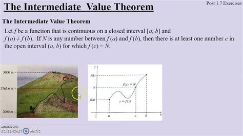
Table of Contents
Mean Value Theorem vs. Intermediate Value Theorem: A Deep Dive
The Mean Value Theorem (MVT) and the Intermediate Value Theorem (IVT) are two fundamental theorems in calculus that deal with the behavior of continuous functions. While both relate to the values a function takes on an interval, they address different aspects and have distinct applications. This article will delve into a detailed comparison of these theorems, exploring their statements, proofs, geometric interpretations, and crucial differences, along with illustrative examples to solidify understanding.
Understanding the Intermediate Value Theorem (IVT)
The Intermediate Value Theorem states that if a function f is continuous on a closed interval [a, b], and k is any number between f(a) and f(b), then there exists at least one number c in the open interval (a, b) such that f(c) = k.
In simpler terms: If a continuous function starts at one value and ends at another, it must pass through every value in between. Imagine drawing a continuous curve without lifting your pen; it must cross every horizontal line between its starting and ending points.
Geometric Interpretation: The IVT guarantees the existence of a point on the curve where the y-coordinate is equal to k. This is visually intuitive – a continuous curve cannot "jump" over a horizontal line.
Formal Statement: Let f be a continuous function on the closed interval [a, b]. If k is a number between f(a) and f(b), then there exists at least one number c in (a, b) such that f(c) = k.
Proof of the Intermediate Value Theorem
The proof of the IVT typically relies on the completeness property of real numbers (every bounded set of real numbers has a least upper bound). A rigorous proof would involve constructing a sequence of nested intervals and using the completeness axiom to show the existence of c. However, the intuitive geometric understanding is often sufficient for practical applications.
Applications of the Intermediate Value Theorem
The IVT has numerous applications, including:
- Finding roots: Demonstrating the existence of a root for a continuous function within a given interval. If f(a) and f(b) have opposite signs, then there must be at least one root in (a, b). This forms the basis of many numerical root-finding algorithms.
- Showing the existence of solutions: Proving the existence of solutions to equations, particularly in situations where an analytical solution is difficult or impossible to find.
- Establishing properties of functions: Deriving properties of continuous functions, such as demonstrating the existence of fixed points.
Understanding the Mean Value Theorem (MVT)
The Mean Value Theorem asserts that for a function f that is continuous on a closed interval [a, b] and differentiable on the open interval (a, b), there exists at least one point c in (a, b) such that the instantaneous rate of change at c, given by f'(c), equals the average rate of change over the interval [a, b].
In simpler terms: There is at least one point in the interval where the slope of the tangent line is equal to the slope of the secant line connecting the endpoints of the interval.
Geometric Interpretation: The MVT states that there exists a point on the curve where the tangent line is parallel to the secant line connecting the endpoints (a, f(a)) and (b, f(b)).
Formal Statement: Let f be a continuous function on the closed interval [a, b] and differentiable on the open interval (a, b*). Then there exists at least one number c in (a, b) such that:
f'(c) = [f(b) - f(a)] / (b - a)
Proof of the Mean Value Theorem
The proof of the MVT relies on Rolle's Theorem, which is a special case of the MVT where f(a) = f(b). Rolle's Theorem states that if a function is continuous on [a, b], differentiable on (a, b), and f(a) = f(b), then there exists at least one c in (a, b) such that f'(c) = 0. The MVT is then proven by constructing an auxiliary function that satisfies the conditions of Rolle's Theorem.
Applications of the Mean Value Theorem
The MVT has significant applications in various areas:
- Estimating function values: Providing a bound on the difference between the function value at two points.
- Analyzing rates of change: Studying the instantaneous rate of change relative to the average rate of change.
- Proving inequalities: Establishing inequalities involving functions and their derivatives.
- Optimization problems: Finding critical points and determining whether they correspond to maxima or minima.
Key Differences Between IVT and MVT
While both theorems deal with continuous functions on an interval, their core differences are significant:
| Feature | Intermediate Value Theorem (IVT) | Mean Value Theorem (MVT) |
|---|---|---|
| Focus | Existence of a specific function value within an interval. | Existence of a point where the instantaneous rate of change equals the average rate of change. |
| Requirements | Continuity on a closed interval [a, b]. | Continuity on [a, b] and differentiability on (a, b). |
| Conclusion | Guarantees the existence of at least one c such that f(c) = k. | Guarantees the existence of at least one c such that f'(c) = [f(b) - f(a)] / (b - a). |
| Geometric Interpretation | The function's graph must intersect every horizontal line between f(a) and f(b). | There's a point where the tangent line is parallel to the secant line joining the endpoints. |
| Applications | Finding roots, showing existence of solutions, establishing function properties | Estimating function values, analyzing rates of change, proving inequalities, optimization problems |
Illustrative Examples
Let's consider examples to highlight the distinct nature of these theorems.
Example 1 (IVT): Consider the function f(x) = x² on the interval [1, 3]. f(1) = 1 and f(3) = 9. Let k = 5. The IVT guarantees that there exists a c in (1, 3) such that f(c) = 5. Indeed, c = √5 satisfies this condition.
Example 2 (MVT): Consider the same function f(x) = x² on the interval [1, 3]. The average rate of change is (9 - 1) / (3 - 1) = 4. The MVT guarantees that there exists a c in (1, 3) such that f'(c) = 4. Since f'(x) = 2x, we have 2c = 4, which gives c = 2. The slope of the tangent line at x = 2 is equal to the slope of the secant line connecting (1, 1) and (3, 9).
Conclusion
The Intermediate Value Theorem and the Mean Value Theorem are cornerstones of calculus, offering crucial insights into the behavior of continuous and differentiable functions. While both are powerful tools, they address different aspects of a function's properties. The IVT focuses on the existence of specific function values, whereas the MVT relates the instantaneous rate of change to the average rate of change. Understanding their distinctions and applications is fundamental for mastering calculus and solving a wide range of mathematical problems. Their practical applications extend far beyond the classroom, impacting diverse fields ranging from engineering and physics to economics and computer science. The ability to apply these theorems effectively is a mark of a strong mathematical understanding and problem-solving skill.
Latest Posts
Latest Posts
-
Select All Of The Following That Are Characteristics Of Plants
Mar 28, 2025
-
What Is The Difference Between Resistance And Impedance
Mar 28, 2025
-
What Structure Controls The Cells Activities
Mar 28, 2025
-
The Process Of Breaking Rocks Into Smaller Pieces Over Time
Mar 28, 2025
-
How To Spell 30 In Word Form
Mar 28, 2025
Related Post
Thank you for visiting our website which covers about Mean Value Theorem Vs Intermediate Value Theorem . We hope the information provided has been useful to you. Feel free to contact us if you have any questions or need further assistance. See you next time and don't miss to bookmark.
